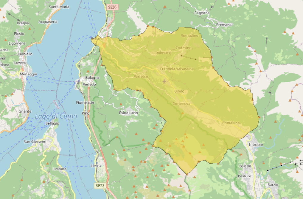
The Project: a landslide survey
Analysis of the east region of Lake Como through Landslide Susceptibility Mapping
STEP 0 - Data download
Firstly we have downloaded the required data:
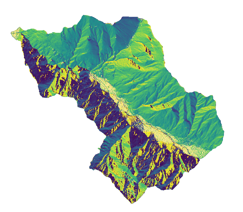
- DTM (Digital Terrain Model): DTM refers to a digital representation of the topography or terrain of a specific area. It provides detailed information about the elevation and shape of the land surface
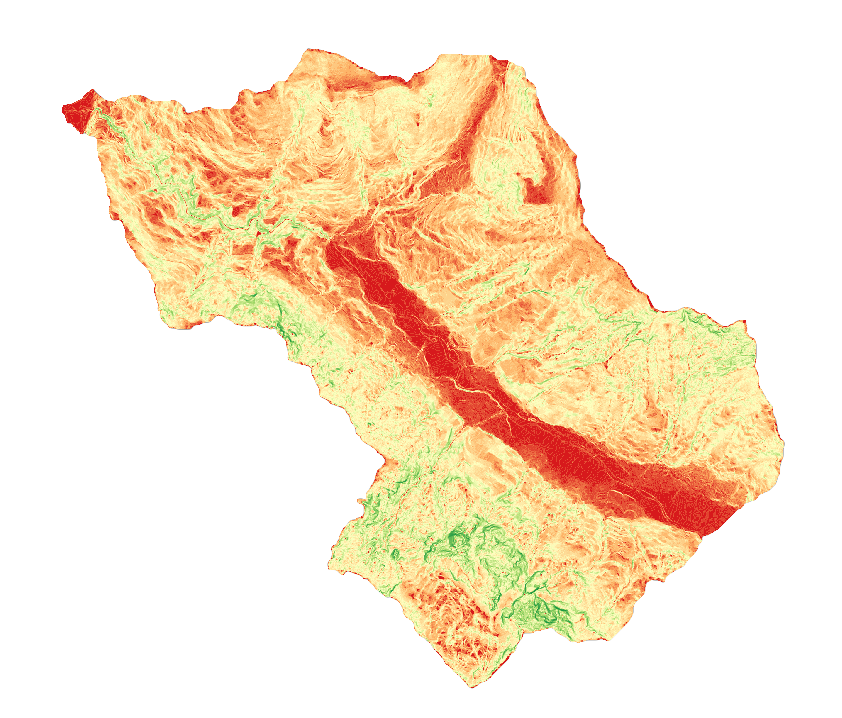
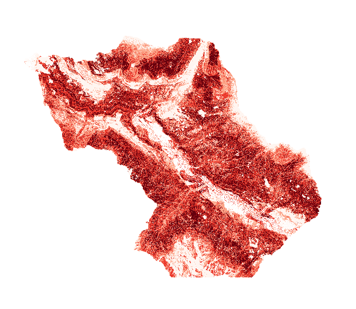
- NDVI (Normalized Difference Vegetation Index): NDVI is a numerical indicator that measures and quantifies the density and health of vegetation in an area. It is calculated using the visible and near-infrared light reflected by vegetation. NDVI values range from -1 to 1, with higher values indicating healthier and more abundant vegetation. In landslide susceptibility mapping, NDVI can be used to assess the influence of vegetation cover on slope stability and identify areas with limited vegetation that may be more susceptible to landslides.
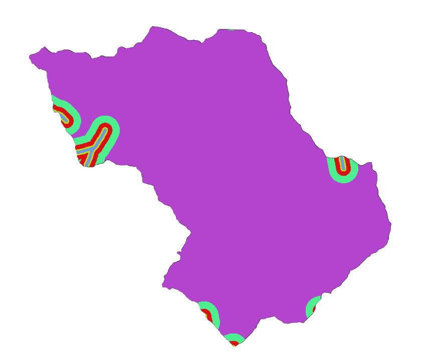
- DUSAF (Digital Urban Surface Analysis Factors): DUSAF can be used to identify areas of urban growth, track changes in urban morphology over time, and assess the impact of urban development on the environment. It consists in a set of factors obtained from high-resolution remote sensing data.
- BUFFER LAYERS OF RIVER, ROADS, FAULTS: The buffer layer is obtained by buffering the original features using a specific distance. This layer is very useful in order to assess relationships between these elements and landslides, helping in evaluating potential impacts.
- LS (Landslide Inventory): It consists in a collection of information related to landslides in a specific area. In our case it is specified the typology of the landslide.
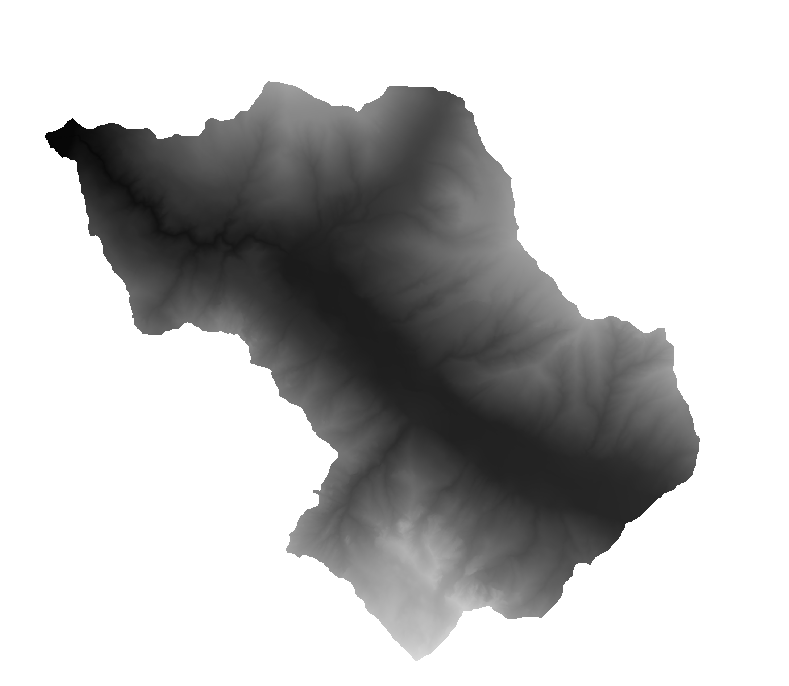
DTM
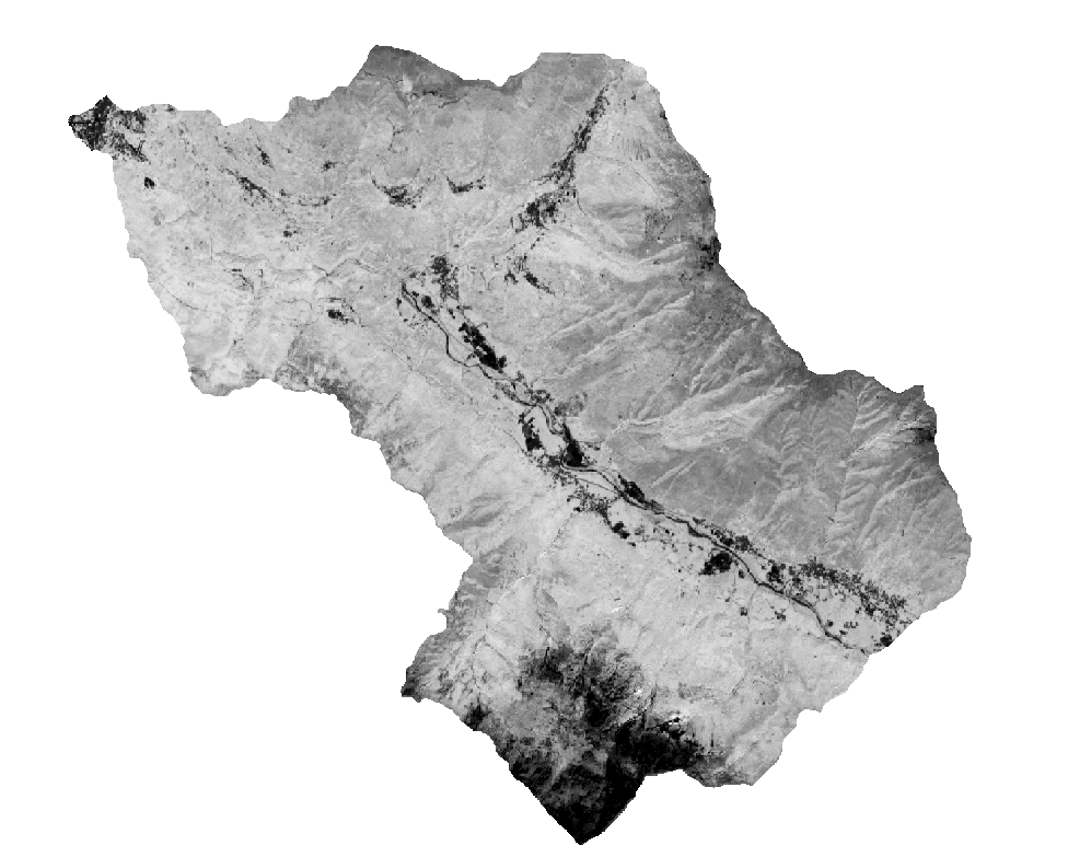
NDVI
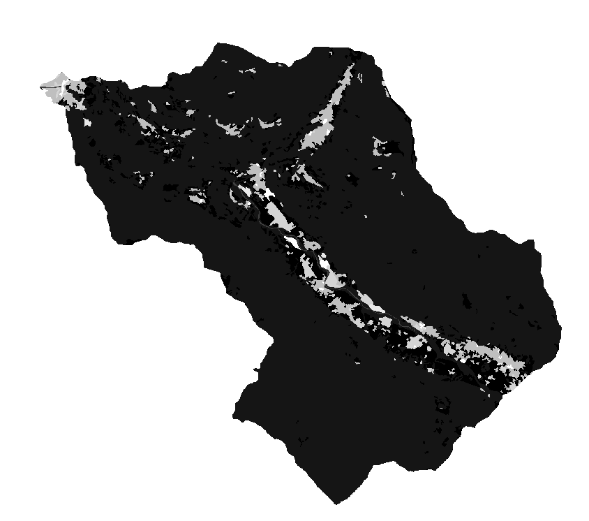
DUSAF
Buffer layers
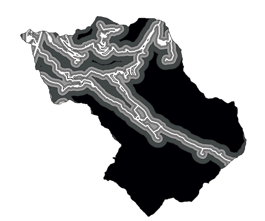
Roads
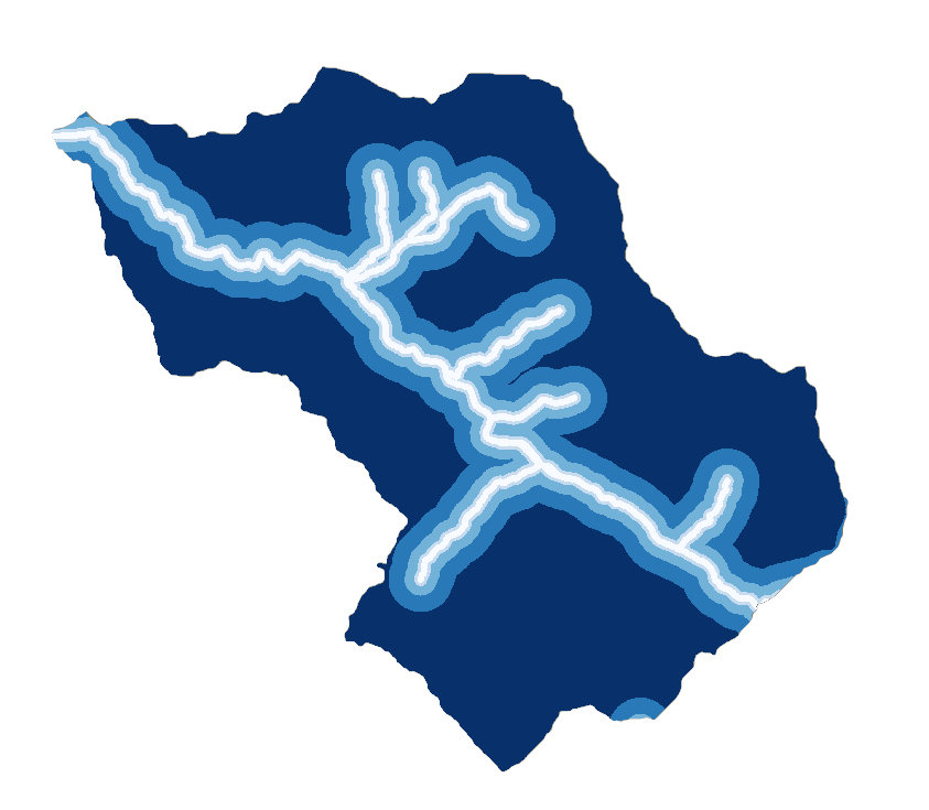
Rivers
Faults
STEP1 - Data preprocessing for susceptibility mapping
- We clipped downloaded raster layers using as mask the vector layer of the group 6 area, using the QGIS Processing tool r.resamp (from GRASS plugin), in order to have, for every raster produced, the same Extent and Pixel Size.
- We clipped vector layers using Clip Vector by Mask Layer (GDAL plugin), using as mask the vector layer of the group 6 area.
After that, we extracted the following environmetal factors by DTM using SAGA plugin.
- SLOPE
The value of the cell in the output slope raster gives the slope value, obtained by calculating the maximum rate of change between each cell and its neighbors. The lower the slope value, the flatter is the terrain; the higher the slope value, the steeper is the terrain.
- ASPECT
The value of each cell in the output aspect raster indicates the direction the cell faces.
- PROFILE CURVATURE AND PLAN CURVATURE
The curvatures highlight the profiles of the slope in both directions, where important classes are the concave which can block a water runoff and augment higher water saturation on the surface and the convex where theaccumulated mass could lead to slope failure.
Aspect
Slope
Profile
Plan
No Landslide Zone
The next phase of the STEP 1 consists in defining the No Landslide Zones, that are those zones of the group 6 area that have slope < 20° or slope > 70°. There are some big NLZ zones, and so it would be convenient to set to 0 negative values and then remove very small patches using the Sieve tool from GDAL. The obtained raster then is vectorized in order to obtain the polygons of NLZ using r.to.vect from GRASS plugin.
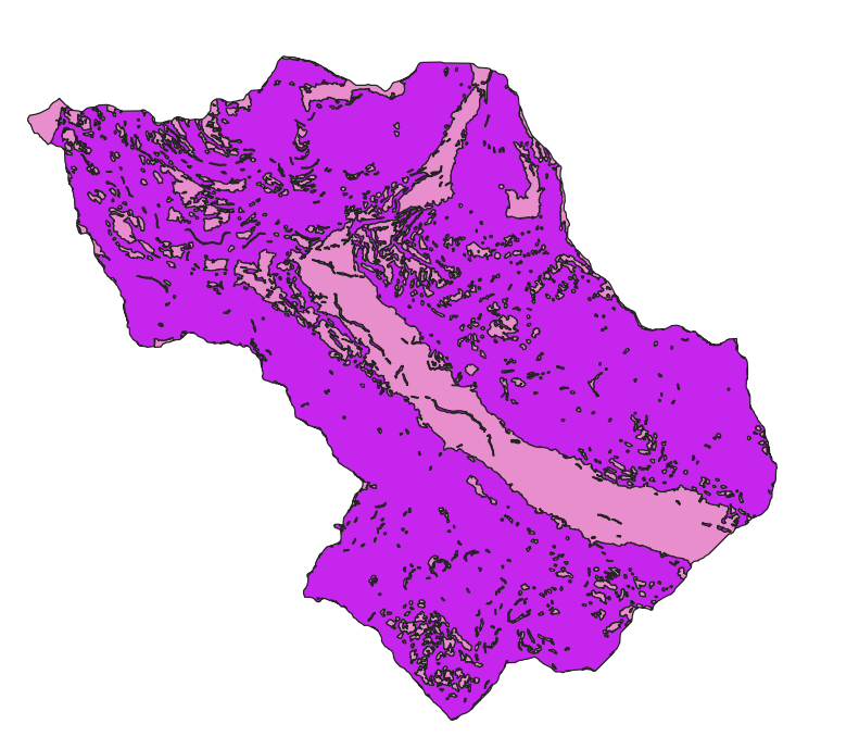
NLZ
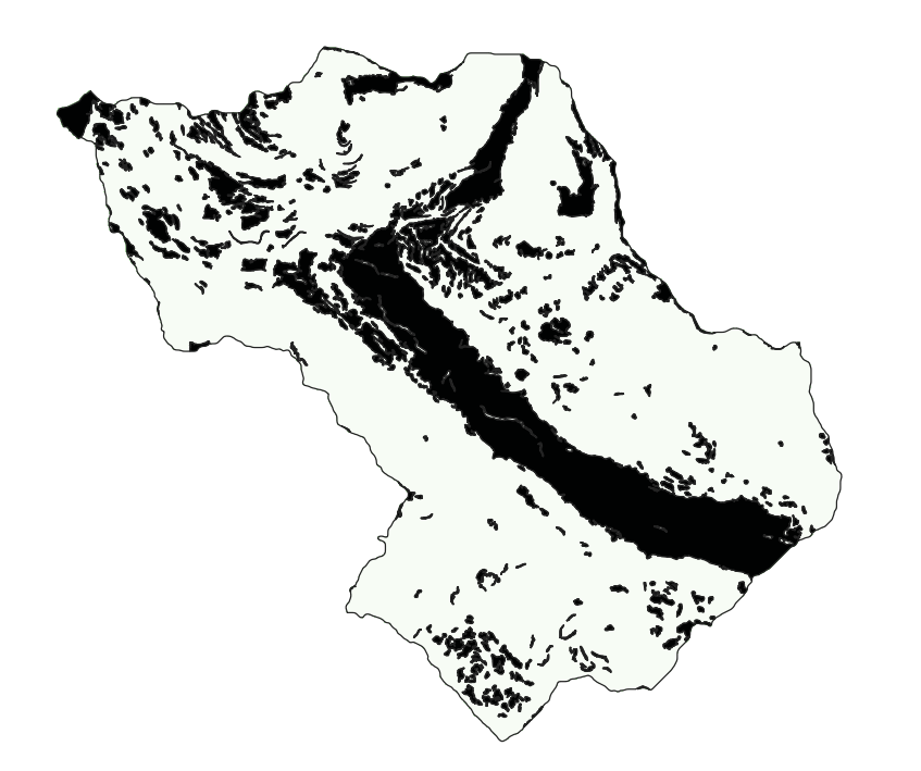
NLZ: bigger patches only
Since the definition of NLZ is simplified (only according to slope) there may be some NLZ areas which overlap the LandslideInventory polygons. For these reason, it is necessary to repear this using the Difference tool that allow to remove from NLZ layer the LS overlapping parts.
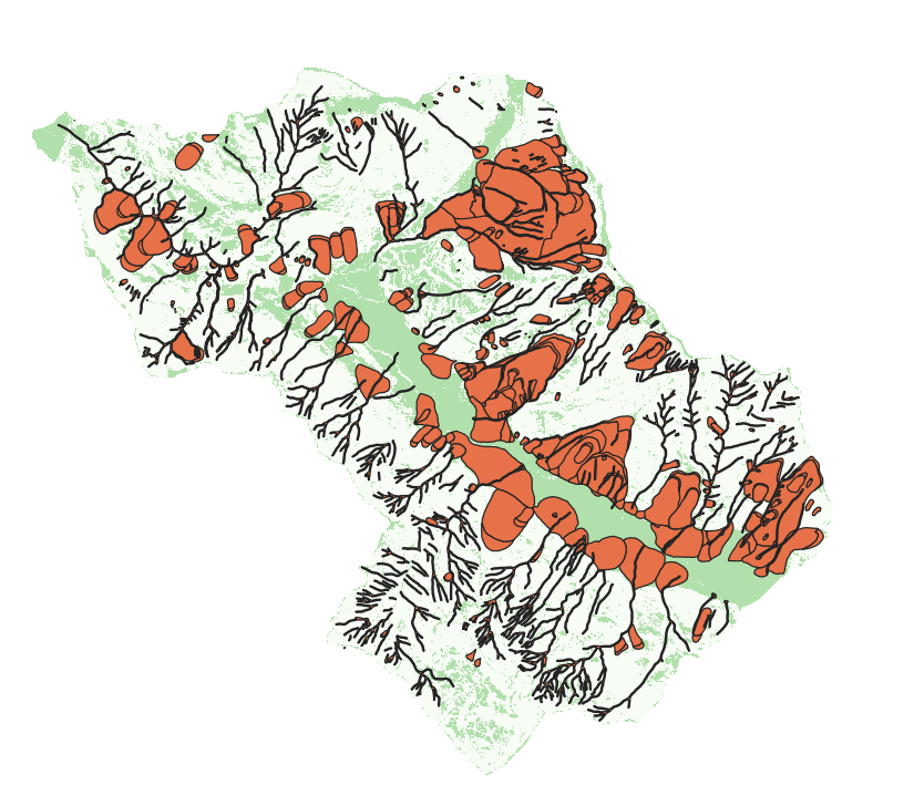
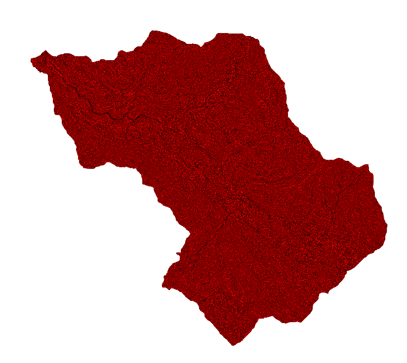
Landslide zone
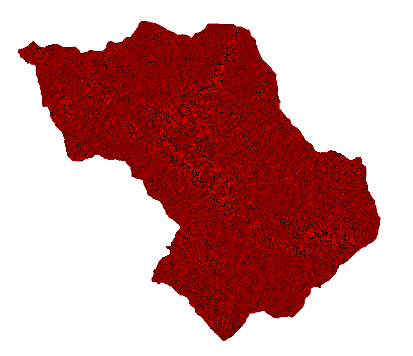
Difference between NLZ and LS
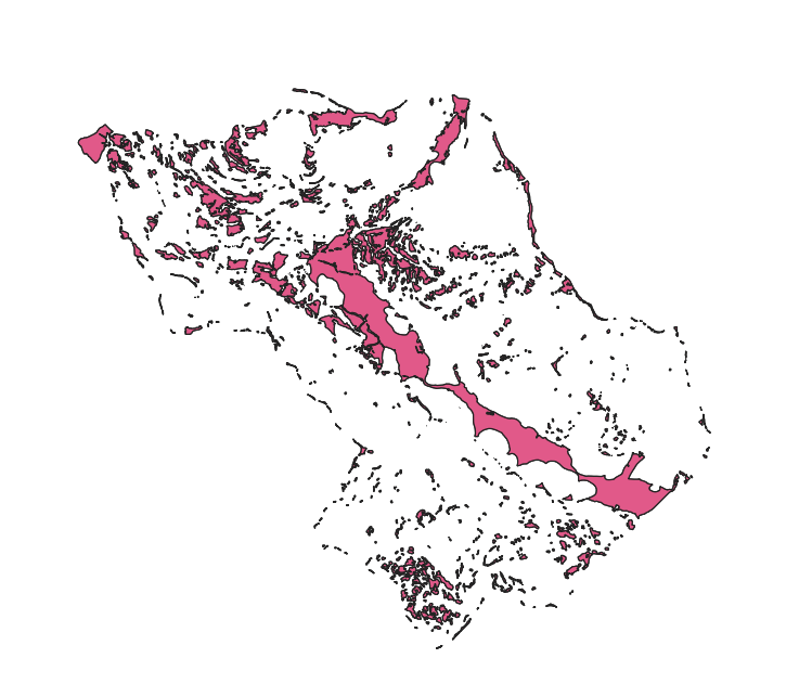
Then, in order to prepare our data to the training/testing phase, it was necessary to add a new field called hazard to the attribute table of NLZ and LS, and then assign value 0 for the attribute Hazard in NLZ, and 1 for hazard in LS.
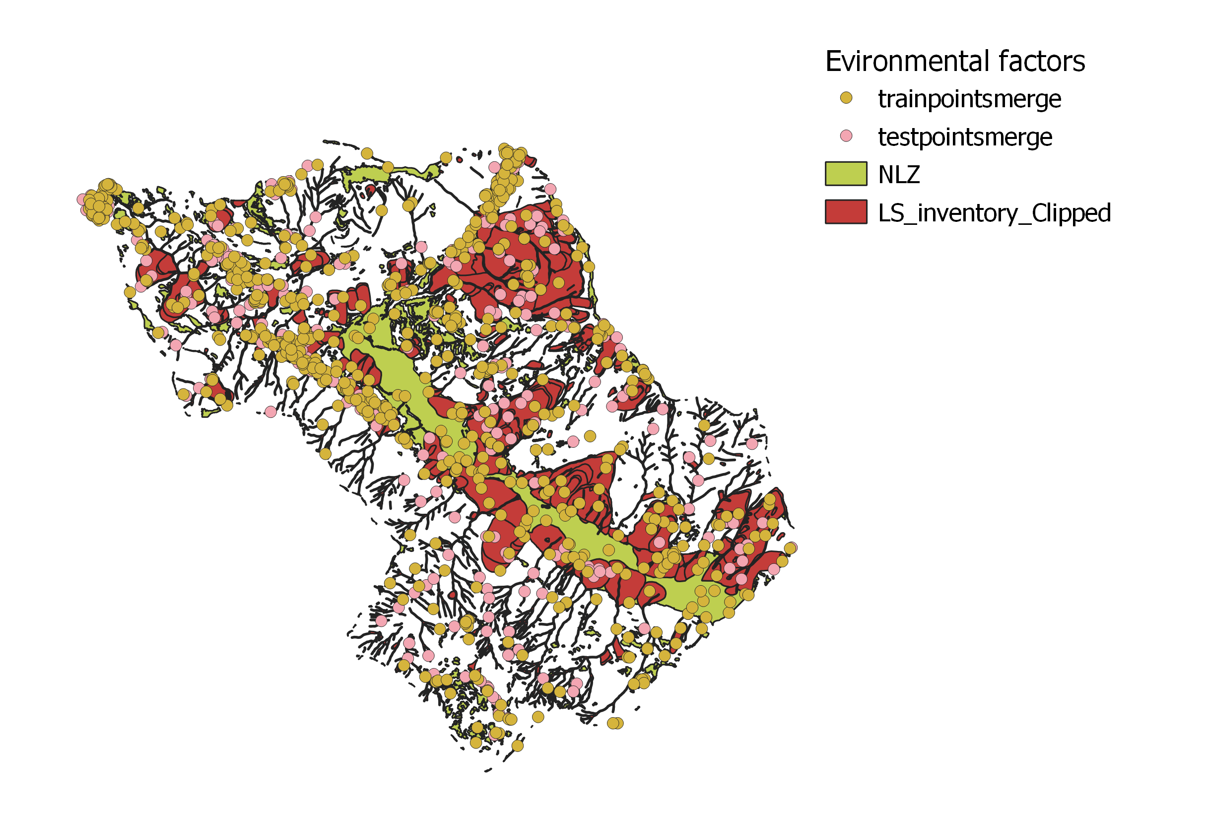
Training and Testing
- We put the training-testing ratio that will be used for the machine learning model equals to 70/30
- For both LS and NLZ we created a new text attribute 'Train_Test', at which is randomly assigned the value 'Training' or 'Testing'.
- We merged the processed LS with the one of NLZ.
- We created random points inside the polygons: the model should be fed with 1000 points, of which 700 for the training phase (350 with 0 Hazard vs 350 with 1 Hazard) and 300 (150 with 0 Hazard vs 150 with 1 Hazard) for the testing phase. For this purpose we used the tool Random Points in layer bounds.
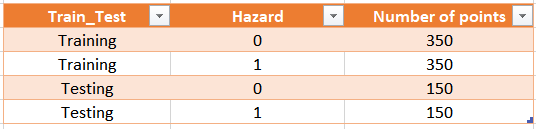
At the end, in order to have a unique layer with training and testing points we use again the Merge tool to obtain trainingPoints and testingPoints layers. These merged layers hasn't any geospatial information connected to them, so it is necessary to sample the environmental factors using the Point Sampling Tool plugin that creates a table with all the useful environmental factors in the selected points. The results will be two layers: trainingPointsSampled and testingPointsSampled with the associated environmental factors.
Outputs of this computation are the following layers:
- dtm.tif
- ndvi.tif
- aspect.tif
- dusaf.tif
- faults.tif
- plan.tif
- profile.tif
- rivers.tif
- roads.tif
- slope.tif
- NLZ.gpkg
- trainingPointsSampled.gpkg
- testingPointsSampled.gpkg
Before starting with the next step, it is necessary to check whether all the output raster layers have the same CRS, extent and pixel size.
STEP2 - Susceptibility Map generation
For the generation of the susceptibility map we used R in QGIS with the ModelMap given script.
Once the susceptibility map has been generated, the R output should be validated: the resulted layer is reclassified in 2 classes, 0 and 1, using Accuracy Assessment and Sampling tool.
The outputs obtained are the Susceptibility Map and the Error matrix.
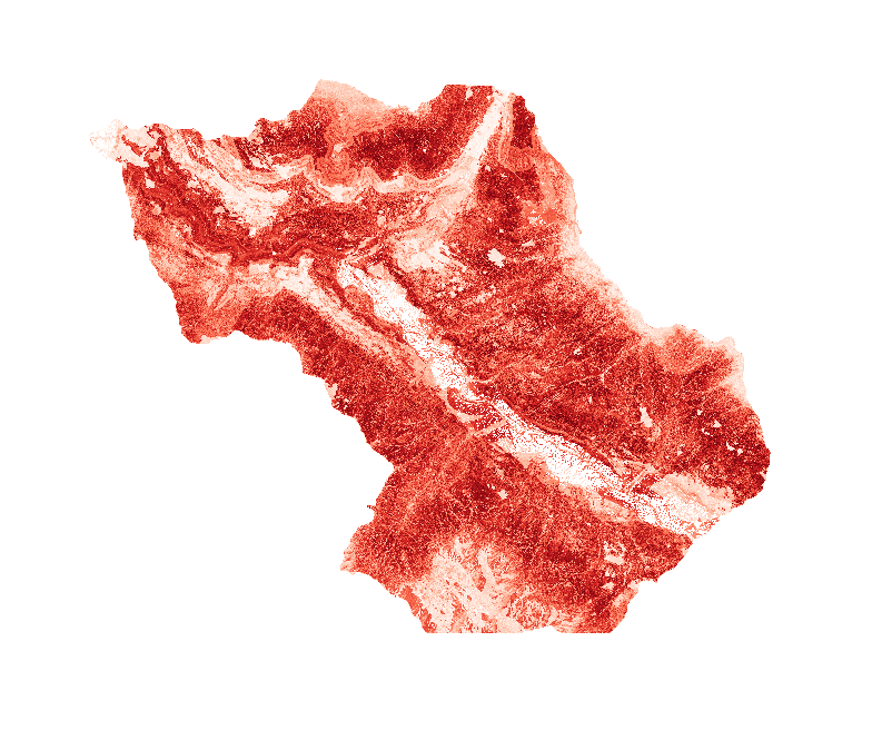
Susceptibility map
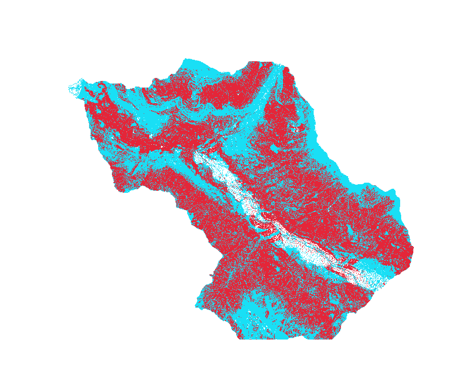
Susceptibility map classified in 2 classes
STEP3 - Data PreProcessing for exposure assessment
After downloading the population raster dataset from WorldPop, we reprojected this dataset using the same CRS of the group 6 area and of the susceptibility map. Then we clipped the reprojected population raster dataset using as mask layer the group 6 sub area.
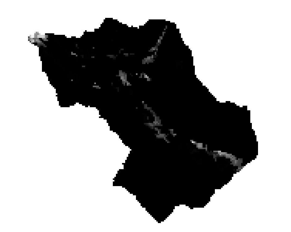
Population
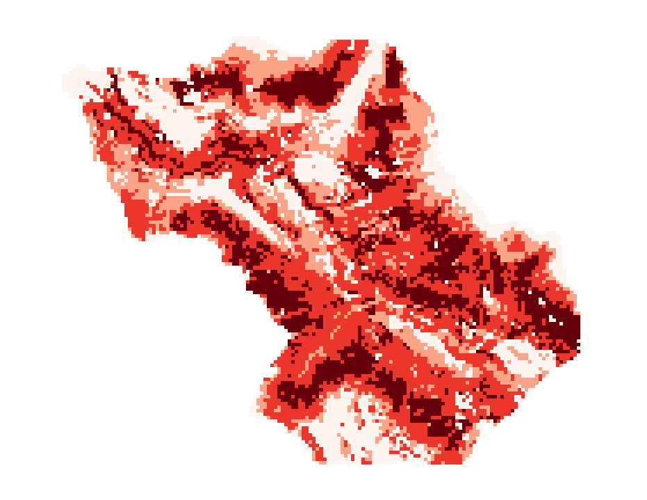
At this point, the susceptibility raster map is classified using 4 different classes of risk (low, moderate, high, very high), obtaining a reclassifided susceptibility map. After that, we resampled it using r.resamp.stats, setting the mode as aggregation method, and the pixel size equal to the one of the population raster.
The output of this step consist of:
- Reprojected and clipped population raster dataset in GeoTiff format
- Reclassified and resampled susceptibility raster map in Geotiff format
Susceptibility map classified in 4 classes
Susceptibility map resampled
STEP4 - Exposure assessment
Exposure assessment is a process used to determine the potential impact and vulnerability of assets, populations, or ecosystems to various hazards or risks. It involves evaluating and quantifying the elements at risk in a given area, such as buildings, infrastructure, natural resources, and people, to understand their susceptibility to potential hazards.
In this step for each one of the susceptibility classes has been computed the population count.
The output of this step is the table with the computed population in each susceptibility class.
STEP 5 - Website and WebGIS development
As a final step, we have developed a WebGIS application that enables users to visualize the analyzed maps and the landslide susceptibility map. Our intuitive interfaces and interactive functionalities allow navigation, zooming in and out, toggling different layers, and accessing supplementary information. These features enhance users' understanding of the landslide susceptibility assessment and the related spatial data.
In addition, our WebGIS platform offers a selection of base maps to choose from, including:
- OpenStreetMap
OpenStreetMap (OSM) is a collaborative mapping project that creates and provides free geographic data and mapping to anyone who wants to use it. It relies on a community of volunteers who contribute data such as roads, buildings, and points of interest. OSM is known for its global coverage and detailed informations.
- Stamen Toner
Stamen Toner is known for its minimalistic and high-contrast black-and-white appearance, resembling traditional printed maps. It aims to provide a clean and visually appealing representation of geographic features, focusing on road networks, labels, and boundaries.
- Stamen Watercolor
Stamen Watercolor adopts a unique artistic style inspired by hand-painted watercolor artwork. It uses subtle colors, textures, and brush strokes to depict landforms, vegetation, and water bodies. Watercolor maps are highly distinctive and are often used for artistic or aesthetic purposes rather than precise geographical reference.